The Bet is Round

The past couple posts have been qualitative in nature and I thought I would spend this time to discuss a foundational component of how I modeled the World Cup, about 5,000 times per model version, discussing how to simulate an event incorporating an element of chance.  I understand not all of you will be interested in sports.  And I understand soccer may not be your cup of tea so I’ll do a couple examples for different facets of life.  Modeling randomness can be a great tool.  Sports.  Personal Finance.  The weather.  Chance is everywhere.  Modeling randomness can be learned and practiced!  In the end it will allow you to make better decisions given certain assumptions.  The assumption setting is a story for another day and most likely requires some background research.  That being said many of us don’t even make decisions based off of what we believe in!  Isn’t that foolish?

There will be a financial example a tad later but we will begin with some soccer simulations.  Let’s start with one matchup, a battle of some of the big boys in England, Arsenal and Liverpool.  In the below setup we are accounting for three outcomes:  1) An Arsenal Win, 2) A Liverpool Win, and 3) A Tie.  In column F you can see the given probabilities of those outcomes.  In the second chart I show the formulas in each cell (how you would actually type them in).  A few things to notice:

1. The important non zero inputs are F3 and F4.  This is where we are getting the win probabilities for Arsenal and Liverpool respectively.  The tie is the complement of the sum of those two win percentages.
2. You can think of the cumulative probabilities as just stacking the three probabilities on top of each other step by step (you’ll see why we need this soon)
3. We are giving Arsenal a 45% chance to win, Liverpool a 25% chance, and the resulting 30% for a tie (this may be slightly biased as I’m an avid Arsenal fan).

With the formulas shown:

Once we have our initial assumptions we need to find a framework to simulate.  In the next couple of panels we will utilize the rand() function in Excel.  With this function Excel randomly generates a number greater than or equal to 0 and less than 1.  We are going to assign a result (Arsenal Win, Liverpool, Win, or Tie) based on the random number generated.

Where do the cumulative probabilities come into play?  We will utilize our cumulative probabilities for the mapping between the random number and the result.  If the random number is less than .45 that will be an Arsenal win.  If it’s less than .7 but greater than or equal to .45 that will be a Liverpool win.  And if greater than or equal to .7 that will be a tie.  Mathematical mappings could be stated as:

[0 , .45) -> An Arsenal Win

[.45 , .7) -> A Liverpool Win

[.7 , 1) -> A Tie

 

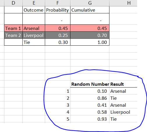
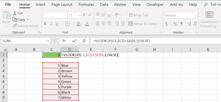
In this example we have five simulated games but the same principles apply to larger samples.  I want to implore you to look into the Index() and Match() functions.  While they can resemble a VLookup() function (my third blog post has more information on that function if you’re interested) their combination enables more versatility.

Couple things to tinker around with:

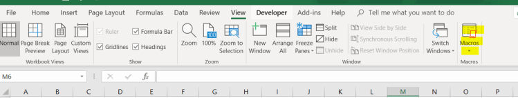
1. Go to an empty cell in the spreadsheet and click the Delete key.  The random numbers should change and thus will alter the results.  If the random numbers aren’t changing check to see if your calculations are set to Manual under Calculation Options (highlighted below).
2. View how the results change every time you recalculate the cells.
3. Now try to run it for 2,000 simulations.  Do the results seem more predictable?

 

Money Example!!!

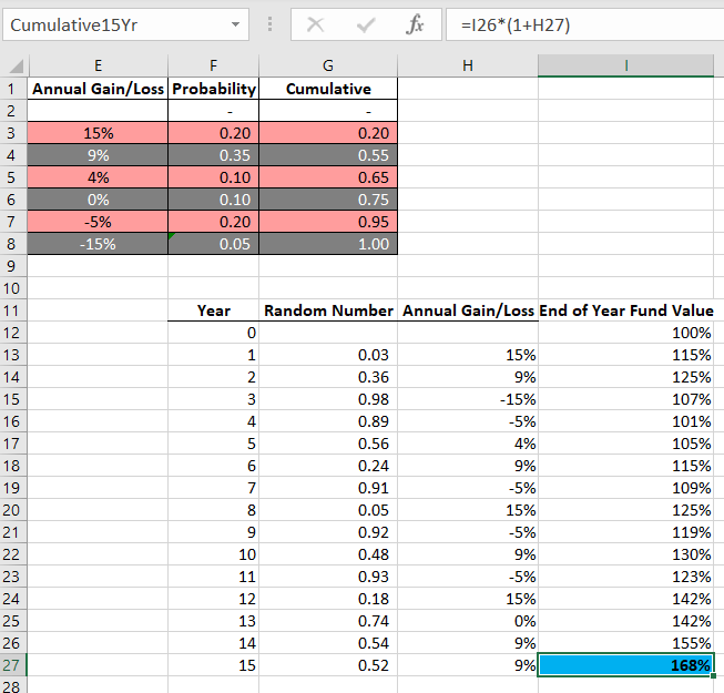
Now we’re going to take the same principles and apply them to a theoretical index fund.  Here instead of assigning probabilities to a certain team winning or losing we’ll be assigning them to a certain gain/loss of the index over the year.  We’ll then apply each year’s return/loss to the prior years and eventually get to the end of year 15.  Our goal in this example is to capture the ending value of the 15th year for 1,000 different simulations.  Depicting those 1,000 ending values in a histogram would be marvelous!

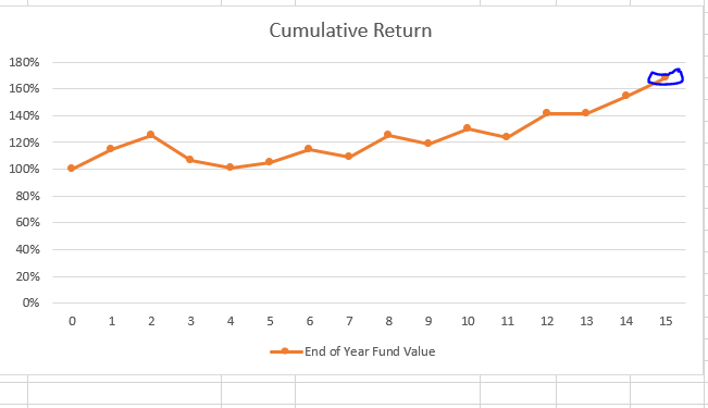
Hopefully the probability table below looks familiar.  Instead of having three game outcomes, as in the soccer example, we have six possible annual returns, in column E.  In column I we have the ending year index value.  In this example we are building on the prior year’s fund value.  For example the end of year three is, in the example below, 1.15*1.09*.85 = 1.07 (cell I15).  Remember we’re interested in year 15 and also keep in mind this is just one simulation; our goal is to look at 1,000 simulations of the 15th year!  I decided to name the 15th year ending fund value, “Cumulative15Yr”.  Why do you think that specific cell is named?

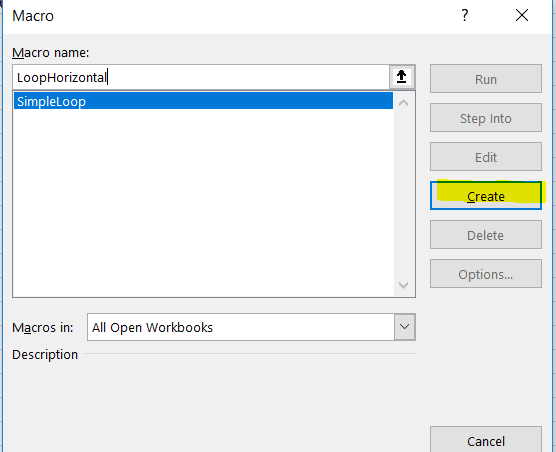
We need to somehow record 1,000 simulations!  Ugh, that’s so tough!  Wait, what tool would be useful for doing a very very very repetitive task over and over and over and over again?  You know this, think!  Back on blog post 2, “Simple Loop in VBA”, we looked at the construction of such a beastly, time saving, and dominating tool.

Instead of copying the 15th year 1,000 times in a column somewhere let’s let the loop do the work for us, and use that saved time to go make a snack (you deserve it).  And remember Pro Tip: Name your important cells!  In this case it was the 15th year fund value.  I, just a personal preference, like to name the cell that will be our anchor to list out the results, wait for it….  Anchor.  Genius I know.

In this VBA loop below we record the 15th year fund value, recalculate the random variables to get a new path of our fund values, and then once again record the 15th year fund value.  The code is so tiny and yet so powerful.

Execute the code and you’ll see something like this appear below the Anchor cell, recording 1,000 ending fund values:

And the very last part we’ll highlight our returns and make a histogram:

There are all sorts of ways to slice and dice this data but this process allows you to see methodically if you believe A) that the index returns have that given distribution then B) you’ll get a distribution of the 15th year fund value looking something like what we obtained.

Fun Tinkering/Thought Ideas:

1. Look at the ending fund value over a longer time horizon like 20, 30, or 50 years.  How do you think that’ll affect the distribution?
2. Try doing 5,000 simulations instead of 1,000.  How did that change things?
3. Mess with the probabilities and returns.
4. Include a large loss but low probability event.

 

Questions/Feedback can be sent to jackallweil@gmail.com and if you sign up on the email list I can send you a pdf of The Bet is Round.

 

It does not matter how slowly you go as long as you do not stop. – Confucius

November 6^th, 2016, is a day that will live with me forever.  My boss called me into her office and there was a stone still HR woman, shoulder pads and all, sitting in the corner of the room with slight disappointment, and moderate sadness, on her face.  I knew this wasn’t warm fuzzy news.  I will admit to having mentally checked out months ago, when just in a little over a year I was working under my third different boss.  I would even say that after the second boss I started just going through the motions.  Simply put, life at Scottish Re was tough and not going well.  I was working as an associate actuary doing valuation related activities at a reinsurance company.  While I’m sure you think it is truly thrilling and would pounce at the opportunity to ask me all sorts of questions I would respond with a calm, “please, cool your jets.”

I was about to get fired, or I was about 99.9% sure of it.  One did not need to be an actuary to figure out that percentage.  After an awkward pause of my boss looking at the hr woman my boss got things rolling, “Jack, it’s just not working out and you will no longer be an employee of Scottish Re.  This is effective immediately.  Do you have anything to say?”

I thought that was a bizarre thing to ask.  Um, I’m sorry?  Thank you I suppose.  What was I to say to that?  The only thing that was going through my head was, ‘damn, if only they could have done this like a week ago I could be in north London watching my beloved Arsenal play their rivals Tottenham in one of the greatest football rivalries.  And I don’t mean American football.  Arsenal, the Kings of London, or more commonly known as the Gunners, were my favorite sports team on earth and the thought of football brought me, albeit only a fraction of a second, some relief.

As a youngster we did not get to watch a lot of European football matches as there was no NBC Sports tv package, that plays essentially every premier league game, like there is today.  I was passively a Juventus fan growing up, a team playing in the Italian Serie A.  It was more a product of me admiring Zlatan Ibrahimovic, a giant Swedish renegade that happened to be a fantastic footballer, and their black and white chic jersey design than me having a real connection to Juventus.  When Juventus got hit with a match fixing scandal in 2006, I was a junior in high school at the time, Juventus was banished to Serie B and Zlatan took off to Inter Milan.  I was left seeing him play only rarely and it felt wrong cheering for Inter Milan.  Another thing happened in 2006 that caught my attention and didn’t feel so wrong.

It was the USA’s first World Cup game in Germany against the 7^th ranked Czech Republic team.  The Czechs had a Juventus player in Pavel Nedved who was world class but the rest of the Czechs were total unknowns to me.  My buddies and I were sitting in a Buffalo Wild Wings in Bay City, Michigan excited for the first five minutes only to be deflated upon the Czechs scoring off a header.  About thirty minutes later I saw a goal that would, no joke, change the trajectory of my life.  This little Czech guy with long brown hair, blue Nike shoes, absolutely cranked a ball from about thirty yards out.  He was on the left side of the field and the ball screamed through the air and went into the upper right corner of the goal leaving the goalkeeper zero chance of saving it.  The little Czech man’s reaction was one of just uncontrolled joy as he outstretched his arms to welcome the hugs of his teammates.  This dude was total class personified and I still feel tears coming on when I watch that play.  His name was Thomas Rosicky and after that World Cup he would be transferred from Borussia Dortmund, in the German Bundesliga, to Arsenal, in the English Premier League.  The rest is history.

I took a deep breath and exhaled, staring at the round table between my boss, the hr lady, and me as it was hard for me to look them in their eyes, “I have to say I feel quite relieved.  I could tell something was off with me being here.  Thanks for the opportunity I suppose.”  A few short moments later, after signing some release forms, which included a generous severance, I realized I would not be coming back here.  And while I was scared some I also felt liberated.

Little did I know that this firing would set off a chain of events that would change my life forever.

At the end of 2016, after my newly found love for reading coupled with a ton of time, as I didn’t have a job, I began to generate more and more ideas.  I was sucked into a black hole of soccer books.  It seemed after I read one I needed to read them all.  Money and Soccer, Soccernomics, 12 Yards, Das Reboot, I am Zlatan, Messi, and My Turn.  They were all great for their different reasons but the two that really changed some of my thinking were Soccernomics and Money and Soccer.  They were written by these two guys who really analyzed the game, and the influencers behind the game, and came up with some insightful findings.  Simon Kupir was more of a cultural writer and did a lot of the Dutch soccer stories including The Dutch, The War which was about the Dutch club Ajax during World War II.  The other guy was Stefan Syzmanski.  He was an English bloak who oddly enough worked in the Kinesiology department at the University of Michigan, where I went to school, and did most of the analytics for these research projects.

Soccernomics and Money and Soccer are an extension of each other in my mind.  They are so blended in my mind that from here on out when I say Soccernomics I could mean either Soccernomics or Money and Soccer.  Soccernomics had a section where they were trying to answer the question of which country uses their resources best in soccer.  I was mesmerized by the question itself and questioning how someone could measure it.  I suppose I thought it’s either in the culture or it’s not but they made me see things a bit differently.  They were looking at GDP per capita, population, and number of international appearances a country had participated in to predict the goal differential between two countries squaring off on the international stage.  They were looking at countries that outdid the goal differential they were predicted by a country with their resources. 

After being in Iceland with my brother in 2016 and seeing all the soccer fields it didn’t really strike me as surprising that Iceland scored well in the Soccernomics analysis.  With only some three hundred thousand people it was amazing they could compete with the likes of the best in Europe.   The old Yugoslavian countries, like Croatia and Serbia, also scored well.  I was very intrigued by this.  Although they found those three factors only accounted for about 25% of the goal difference that got my mind spinning.  What else might be able to help predict goal difference?

I was determined to talk to Syzmanski.  I called him multiple times at the university to talk to him and maybe get some insights or help.  Four times I tried to call him with no pick up and no reply.  I thought about throwing in the towel but called a fifth.  No response.  What was this guy doing?  Was he so busy he really couldn’t pick up my call?  He was a professor, not the President of the United States.  Sixth time, winner winner chicken dinner!  I was actually surprised when he picked up the phone.  It was almost turning into one of those times where you’re calling a pretty girl and slightly hoping they don’t pick up so you can just leave a message and to at least tell yourself you tried.  Please don’t tell me I’m alone on that sentiment. 

I started telling him that I loved his book and I’m guessing he doesn’t get many fan calls.  Kurplop, I heard him drop his notepad or maybe even his laptop.  I won’t go as far as to say he sounded in shock, but I would say legitimately surprised.  “Oh really?”  he asked.

He was very eager to help me and oddly curious as to what I was all about.  “Where are you from?”  he asked.

“About 100 miles north of Detroit on Lake Huron.  It’s a super small town, Linwood, just north of Bay City and Saginaw, you may have heard of those.  But I went to Ann Arbor for school and lived there 3 years while working as an actuary in one of the Detroit suburbs.  I thought it was a cool coincidence when I saw you worked at U of M.”

He replied, “oh, I’m sorry you’re from there.”  That was a slightly dickish thing to say but I’ll let it slide even though it didn’t sound entirely playful.  I perfectly liked where I grew up.  I just got a bit tired of being so cold. 

I started explaining to him what I was thinking about doing.  I wanted to start looking at factors that could help me predict goal difference and in turn help predict the chances of team A beating team B.  I would then look at what the Vegas odds were compared to what I was predicting and purchase the bargain picks, or at least take my chances on the bets that weren’t a complete rip off.  I was looking for value, maybe Portugal paying $1.80 for every $1 to win their group was a super bet, or maybe Iceland getting out of Argentina’s group with getting $2.5 for every $1 bet. 

“Here let me get something.  I have my sources written somewhere over here.” 

Say what?  He was going to give me his sources?  Damn this was so easy!  One phone call, that’s all it took.  Well really six phones calls is all it took. 

Syzmanski continued, “So I got all the game scores from a German site called laenderspiel.de but it comes in English too, think also in French.  It’s incredibly comprehensive.  It has all the conference scores, number of international appearances, and FIFA rankings.  The country data is from the world bank database, which should have csv’s going back 50 years, but you’ll have to do a bit of work to break up the UK numbers to get Wales, Scotland, Northern Ireland, and England Data.  So that’s where we got the population and GDP/capita numbers.”

I continued beginning to talk before I finished noting all of his sources, “Wow, this is so helpful.  Yeah, I’ve done a lot of simulations and optimizations for American football and even ran a daily fantasy information site awhile but got scared they’d make it illegal, but I’m very excited to try and do something for soccer.”

“So where are you now?”

“I’m working as an actuary in Charlotte, North Carolina.  I’ve been in Charlotte about two and half years and at this job less than a year.  The weather is very nice but I do miss my family a lot.”

“Well, this is very cool of you to call.  I’m always interested in how our data and books are received and used.  I’d love to see what you end up doing with this.”

“Yeah, I’ll be sure to let you know. Thanks again.”

So my friend came to me this weekend, after having a wonderful Thanksgiving with his family in Virginia, and he was looking like this:

Now some may think possibly:

1. He ate too much
2. He had not been around me in a full week
3. He loves his momma a lot and misses her

But wait I thought.  Does this guy know what a VLookup is?  Maybe that would totally cheer him up.  I started conversating, “Sachin, I think you really need to learn about VLookups, it’s totally changed my life, for the better obviously, and my soccer model that you think is mediocrely cool would not operate without them.”

“Jack, please tell me more!”

“Sachin, I will tell you more.  What if I told you instead of keeping all of those girls’ names, numbers, eye colors (kind of creepy), and other random information in a spreadsheet, that must be at least 300 rows, you could type in a girl’s name once and all that vital information would populate for you.  Would that be something that interests you?  At the top of the page, with you having to do absolutely no scrolling, you could type in a name and all that creepy information you’ve collected would generate for you without having to fumble through your massive table.”

“Yes, that’s exactly what I need in my life!”

“Well sit back my friend, lets get you a good setup.”

What is a VLookup?  A VLookup, or vertical lookup, is an Excel function and is a convenient way to grab data from a table by attempting to match a given value looking down a column, or vertically.  If you wanted to go against conventional practice you could also investigate looking at HLookups, or a horizontal lookup, but that may be too much craziness for one day.

What are the parameters that go into a VLookup function?

• lookup_value is the value one wants to lookup!  It’s the value in the leftmost column in the table you want to do your lookup.  Perhaps, for Sachin, his table has the nicknames of girls as they appear in his cell phone.  After we set this up all he’ll have to do is type that one nickname and then voila!
• table_array is the range of cells that are being investigated.  It’s Sachin’s whole table, including all his rows, starting with nicknames, and accompanying columns with random information.
• col_index_num is the column of the table that he wants to retrieve with this VLookup.  The lookup column is considered 1, not 0 as some may think.  If this were for instance set to 3 then this lookup would:
  • Go down the first column until the lookup_value was found
  • Count over two more columns and retrieve that value
• [range_lookup] is an optional variable.  It’s asking if searching down the column should be an exact match or just an approximate match.  If one wants an exact match one will set this variable to FALSE, which is what I will use in this example and is what I use about 95% of the time.  If one leaves this blank it will default to FALSE.  Approximate matching, or setting this variable to TRUE, can be useful if you have a lookup number that may or may not be one of the numbers in the column but you want to lookup a similar number.  The tricky part about the approximate match is the lookup column numbers in the table need to be in ascending order.  I encourage you to play with this setting later on.

Before we get too crazy with Sachin’s table let’s look at the following example, a 7×2 table with numbers in the leftmost column and colors in the second, and try to answer the following:

1. What is the value being looked up?
2. What is the value that will be returned?
3. What would happen if col_index_num was set to 2 instead of 1?
4. What would happen if col_index_num was set to 10 instead of 1?

Answers:

1. 2.  This function will look down column C and look for a 2.
2. It’s not very exciting but it will return a value of 2, which is the same as our lookup value.  This is not all that practical but it starts to paint the picture for what this function can do.
3. The function would return Brown.  It would look for the row that has a 2 in the leftmost column and then go to the second column of the table and return that value.
4. You can’t do that!  And Excel will let you know by returning a #REF! error.  The REF is short for reference and tells us we need to check our reference to some of our values we’re using.  Our table only has two columns but we’re asking to send us back the 10th column in the table.  We’d either have to adjust our table or adjust the col_index_num to eliminate that error.

Let’s now start looking at Sachin’s table that he’s started constructing with some VLookups setup at the top:

Here Sachin has started constructing his table.  He says he has many more names to add but I’m starting to question the validity of this list as many of the last names are eerily resembling my fantasy football team players:)

But you’ll see now he can just type in a nickname, how he originally typed it into his phone, in the green C2 cell.  Row 2 is a bunch of VLookups that look through the table and bring back a specific column of information relating to that lookup value.  In our original VLookup example the col_index_num value was an integer but we’ve made that value a dynamic value that can change.  The VLookup formula in E2 is actually looking to E1 to get its value for col_index_num.

This may be easier to see by looking at a different lookup cell and with a different lookup_value.  We’re now looking for information relating to “Uber Girl”:

You’ll notice D2 through I2 update with new information as C2 gets changed.  While this is a small glimpse into the power of the VLookup I hope you can start seeing the use if you had 100’s or 1000’s of rows in a table with many more columns, and maybe more productive (some would say) information.

Sachin is well on his way to living that good life and is now looking like this:

While the fun and games are temporarily over it doesn’t have to last long.  If you sign up for my email list I’ll send you a copy of “The Bet is Round” for free in pdf form, where I map my crazy adventure into betting on the 2018 FIFA World Cup.  I’d love to hear your feedback.

 

“Nothing ventured, nothing gained”